One Look-Up Function to master (Index & Match)

One Look-Up Function to master (Index & Match), In today’s article the focus are on one of the best lookup function. Index and Match combined are an incredibly flexible way to look up data. Attached to the Article you will find a PDF version for printout. There is also an Excel file that have one sheet containing a dataset (booklist with columns author, title and ISBN) and a task part containing 4 columns; Task, Search Criteria, Your Test and Answer.

You can test yourself by entering the code described further down in this article into column C, “Your Test” in the attached Excel sheet. In Column D, answer you will see what result you’re supposed to get.

It is for sure no understatment that One Look-Up Function to master (Index & Match) increases our utilization of Excel.

Index and Match, what are they and what do they do:

MATCH – This function is used to find the position (row number) of a given search criteria in the dataset we want to get the value from. The purpose of Match is by that to find the row/column coordinate for the value the user is looking for.
INDEX – Returns the contents in a specific row/column intersection based on a position given in its criteria’s (Column and row number). The purpose of Index is by that to return contents of a field elsewhere in the workbook to the field where the user wants it.

When combining these two functions is Match used to find the row number for a certain search criteria and Index to return a value from the same row but different column.

Please use attached Excel sheet for practical training on these functions, snapshot of it at the bottom of the article for field references.

Click here to find useful Excel tips and tricks

How to use Match

The One Look-Up Function; Index & Match is a combination function cosisting as described of the functions Index and Match. The MATCH function searches for a specified item in a range of cells, and then returns the relative position of that item in the range.

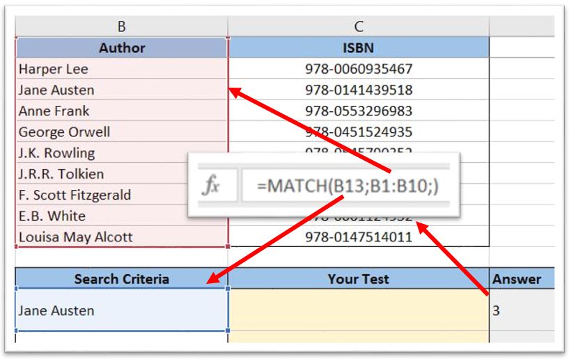
Start by placing the marker in C13. Type in “=Match(“
Select field B13 either by use of the mouse
Enter a semicolon “;”
Select the data range to look in, “B1:B10” by use of the mouse
Enter a semicolon “;”
Type 0 for “Exact Match”
End code with a “)” and press enter
The shown result in C13 should be “3”

Easy and flexible way to find the position of the first occurance of a search criteria. Combined with Index, it is a handy tool for finding corresponding data on the same row as the data searched for.

Click here to learn how to use Microsoft Excel shortcuts

How to use Index

There are two ways to use the INDEX function, If you want to return:
– the value of a specified cell or array of cells.
– a reference to specified cells.

It is the first way that is described beneath, how to find and return the value in a given cell or array of cells based on a set of criterias.

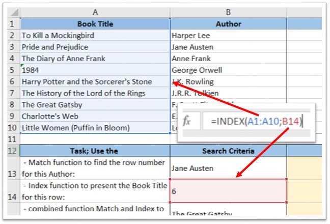
Start by placing the marker in C14. Type in “=Index(“
Select the data range to look in, “A1:A10” by using the arrow keys to move to A1, press and hold shift and then move to A10 with the arrow keys.
Enter a semicolon “;”
Select field B14 by using the arrow keys to move to B14
End code with a “)” and press enter
The shown result in C14 should be “Harry Potter and the Sorcerer’s Stone”

INDEX; the easy function to find and return a value or the reference to a value from within a table or range of data.

Click here to find out how to unhide everything in Excel

How to use Index and Match together

Introduction to Index and Match, To lookup in value in a table using both rows and columns, you can build a formula that does a two-way lookup with INDEX and MATCH.

Start by placing the marker in C15. Type in “=Index(“
Select the data range to look in, “C1:C10”
Type in a semicolon “;” followed by “Match(“
Select field B15 or write B15.
Enter a semicolon “;”
Select field “A1:A10”
Enter a semicolon “;” and “0” for exact match followed by “))”.
Press Enter, given result in C15 should then be 978-0743273565

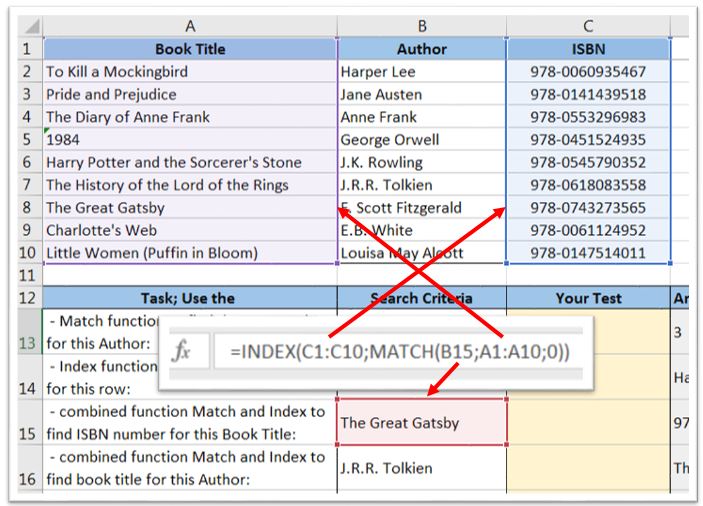
Row 16 to 20 in the attached Excel spreadsheet gives more exercises with Index and Match used together. The only difference from above sample is the search criteria, where we search and what to return. Quite simple, so please feel free to play around with it.

Sum-up:

One of the most popular tools in Excel is the combination of INDEX and MATCH to perform advanced lookups. Together these to functions are incredibly flexible, they can perform horizontal and vertical lookups, 2-way lookups, left lookups, and even lookups based on multiple criteria.

The Index/Match combination is one of the best ways of finding a record in an Excel sheet based on search values. The key benefits is that the data records to be searched does not have to be in sequence. Independent of sorting the function will find the first apperance of the data searched for and return contents from the field asked for.

For improvement of Excel abilities, INDEX and MATCH should be among the first functions to understand and master. One Look-Up Function to master (Index & Match) will for sure give you a strong usefull look-up tool.

Now it is your turn to try it!

Download the file under the Excel icon above and check it out.

More tips and tricks on Office-Tips.net….

Move entire rows & columns in Microsoft Excel

One function that certainly is handy to know is how to move entire rows or columns in Excel. Easily done by drag and drop to the new position.

Stop fussing around when there is need to reorder rows or columns. Use our quick and neat method to drag and drop rows or columns.

Click here to learn a smooth way to drag and drop rows and columns to a new position.

Unhide everything or parts of the data in a spreadsheet.

Change Office menu language (Microsoft Office)

There are several methods and ways to unhide rows and columns in Microsoft Excel spreadsheets.

In this article there is an explanation to more options for unhiding data that can be nice to know.

It describes ways to unhide a selection of rows or columns in addition to unhiding everything.

Click here to learn how to unhide everything or just part of the hidden data in a Microsoft Excel spreadsheet.

Office-Tips.net article overview

Do you wish to read more of our articles about office products? To get a full overview of all Office-Tips.net articles it is just to [click here].

If user guidance to Excel is the topics you are looking for. Then it is just to [Click here]. This page shows an overview of all Microsoft Excel related articles.