The article today is the first explanation for use of a nested Excel function on Office-Tips.net. There are several ways of looking up values in Excel. Our example is by use of three ways to look up a value in Excel by use of functions.
Some examples of look up functions are Find and H/VLookup, but there are lots more listed in the category “Lookup & References” under Functions in Excel.
The example described is a combination function which we find easier and more reliable to use than the standard functions. Our Excel combined function consists of 2 different Excel functions nested together. But no worries they are easy to use and hopefully well explained bellow.
First, which functions do we use in this example:
- MATCH – This function is used to find the position (row number) of our search criteria in the dataset that we want to get a value from.
- INDEX – Returns the value in a specific row/column intersection based on the position (row number) found by use of the Match search and the column that contains the value we want to get.
Attached to this article you will find both an Excel sample sheet and a PDF of this text for printout. In the Excel sample file there is two sheets, one sheet is called dataset. This sheet contains a “100 books everyone should read” list and will be our library to find and get data from.
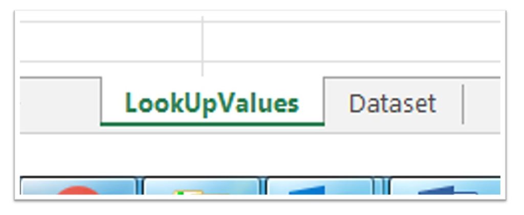
The second sheet in the workbook is called LookUpValues, in this sheet you will find all sample codes used in this article with some more examples including explanation text. Fields with functions in has a soft orange background colour.
In our example we use a book title “Harry Potter and the Sorcerer’s Stone” to find the ISBN number that belongs to the book.
Click here to find useful Excel tips and tricks
How to look up a value in 3 steps:
1. Use of the Match Function
Match is the function that looks for a given value in another Sheet/Column and returns the row number. So belowe is the first of three ways to look up a value in Excel
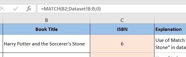
The first code to use, the inner one in our nested example is Match. This is the code in the LookUpValues sheet that gives 6 in field C2. It is shown in the picture to the right and with an example in the attached Excel workbook. The code used is “=MATCH(B2; Dataset!B:B; 0)”.
Explanation:
- “Match” is the function and all criteria’s for the function is separated by semicolon and found inside the brackets.
- Criteria 1, “B2” is the Row/Column intersection that contains the data-record to search for.
- Criteria 2, “Dataset!B:B” in the Match function is the part that routes the search to the complete column B (B:B equals complete column) in the “Dataset” sheet (Dataset! routes the search to the Dataset sheet).
- Criteria 3, “0” in the Match function is an instruction for Match to only find exact matches of Criteria 1, which is the contents of field “B2”.
So, in this case is Match returning number 6, which is the row in the sheet “Dataset” where column B contains the book title “Harry Potter and the Sorcerer’s Stone”.
(Open the Excel sheet, select everything in the Dataset sheet and try to re-order the contents. When doing that you will see that the value in C2 is changing based on which row the book “Harry Potter and the Sorcerer’s Stone” is found.
Click here to learn how to use Microsoft Excel shortcuts
2. Look up a value with use of the Index Function
Index is the function that uses a Column/Row coordinate to look up and return a value.
In Column C and Row 3 of our LookUpValues sheet we use the Index function to find the ISBN number from the Dataset sheet.
Belowe is the second explanation out of three ways to look up a value in Excel.
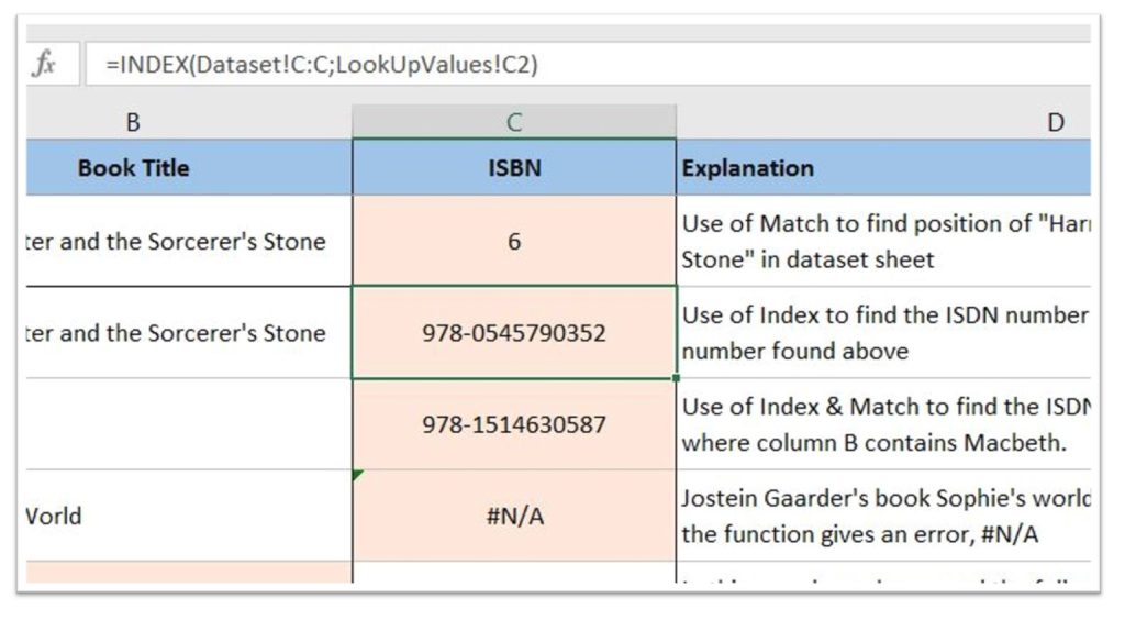
Here we use the value (row number) we found in section 1, Explanation for use of Match Function. The Code in C3 shown in the picture to the right and in the attached Excel workbook is “=INDEX(Dataset!C:C;LookUpValues!C2)”.
Explanation:
- INDEX is the function and all criteria’s for the function is separated by semicolon and found inside the brackets.
- Criteria 1, “Dataset!C:C” instructs the Index function that we only want a record from Column C in the Dataset sheet.
- Criteria 2, LookUpValues!C2 instructs the Index function that we only want contents from the row we found under section 1, the row found was 6.
So, in this case does Index returns ISBN number “978-0545790352” for the book titled “Harry Potter and the Sorcerer’s Stone”. This is the content of intersection row 6/column C in the sheet “Dataset”.
3. How to combine Index and Match to look up a value
The last part is to combine Index and Match. So here is the last of the three ways to look up a value in Excel.
It is straight forward to test this, just replace second criteria “LookUpValues!C2” of the INDEX function with a copy of the complete MATCH function except the equal mark “MATCH(B2;Dataset!B:B;0)”.
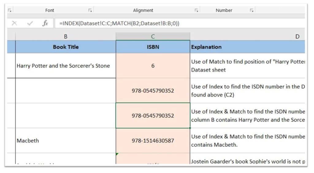
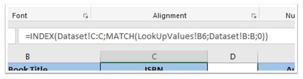
This should give the following code: =INDEX(Dataset!C:C; MATCH(B2;Dataset!B:B;0) )
By that we have made our own search function! The use of complete columns instead of a range of rows inside a column makes the function much easier to move, expand, copy and so on.
Code lines converted into plain text:
The short story for our look up function, this example is found in row 4 in the excel sheet “=INDEX(Dataset!C:C;MATCH(B4;Dataset!B:B;0))” and is described in plain text below:
| Get us the value we’re looking for | INDEX( | |
| Return the Value we’re looking for from this sheet and column: | Dataset!C:C; | |
| Get me the row number where the value we’re looking for is found: | MATCH( | |
| Use the value in this row and column intersection as the criteria: | B4; | |
| Search after the criteria value in this sheet and column: | Dataset!B:B; | |
| Get us only a result when search criteria match perfectly: | 0)) |
This became a little more complex to explain than we foreseen, so a smaller example will follow using one sheet and just some few records. Should make it easier to understand the basics.
But still hope you enjoyed this one and is ready for exploring Index and Match…..
Now it is your turn to try it! Download our file under the Excel icon above and try it out.
More tips and tricks on Office-Tips.net….
Move entire rows & columns in Microsoft Excel
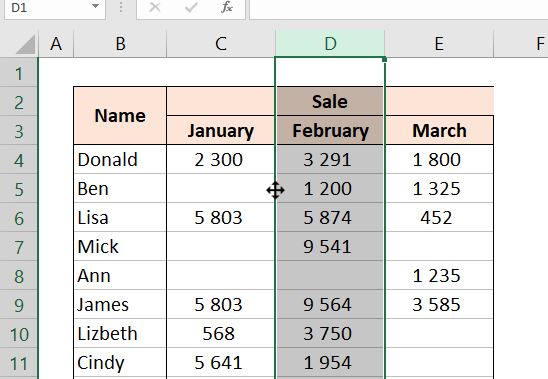
One function that certainly is handy to know is how to move entire rows or columns in Excel. Easily done by drag and drop to the new position.
Stop fussing around when there is need to reorder rows or columns. Use our quick and neat method to drag and drop rows or columns.
Click here to learn a smooth way to drag and drop rows and columns to a new position.
Unhide everything or parts of the data in a spreadsheet.
There are several methods and ways to unhide rows and columns in Microsoft Excel spreadsheets.
In this article there is an explanation to more options for unhiding data that can be nice to know.
It describes ways to unhide a selection of rows or columns in addition to unhiding everything.
Click here to learn how to unhide everything or just part of the hidden data in a Microsoft Excel spreadsheet.
Office-Tips.net article overview
Do you wish to read more of our articles about office products? To get a full overview of all Office-Tips.net articles it is just to [click here].
If user guidance to Excel is the topics you are looking for. Then it is just to [Click here]. This page shows an overview of all Microsoft Excel related articles.